The goal of this practical session is to learn common ways to visualize, filter, analyse and cluster clones on the Vidjil web application. These clones may have been computed by the Vidjil algorithm or by any other algorithm.
This tutorial is composed of three parts: the first one about uploading and managing data from several samples on the platform, and the two last ones about the visualization part for browsing and analyzing clones one one or multiple samples.
You can directly go to the part of the tutorials you are more interested in. Bear in mind that the first part of the tutorial uses a dataset that is provided at the start while the other parts uses a toy dataset already available on app.vidjil.org.
Main help page of the Vidjil platform: https://www.vidjil.org/doc/user
In this tutorial, we will see how to make the best use of the patient and sample database of Vidjil and how to use it efficiently. You need an account on the public server with the rights to create new patients, runs, sets, to upload data and, preferably, to run analyses. Therefore the demo account is not suitable.
1. Go to app.vidjil.org and log in to your account. You can there click on request an account if you do not currently have one. The public app.vidjil.org server is for test or research use. Do not use it for routine clinical data. The VidjilNet consortium offers health-certified options for hosting such data.
2. Retrieve the toy dataset at vidjil.org/seqs/tutorial_dataset.zip and extract the files from the archive.
You should now have three files. We will imagine that those three files are the results from a single sequencing run. More precisely, each one corresponds to a single patient. Thus we now want to upload those files and assign all of them to a same run and each of them to a single patient.
3. Go back to the main page of the Vidjil platform (by default app.vidjil.org). You should be on the patients page. Go at the bottom of the page and click on + new patients to create the three patients.
In a routine clinical setting, you should check whether the patient has already been created by searching her/his name in the search box at the upper left corner.
4. You are now on the creation page for patients, runs, and sets. You can create there at once several patients, runs and sets. Patients, runs and sets are just different ways to group samples. The names are just used to add some semantic so that you know that your patients will be on the patient page, your runs on the run page and your other sets (thus any set of samples you want to make) on the run page. Here we already have a line to create one patient. We want to create two additional patients and one run. Thus click twice on add patient and once on add run.
Now you should have three lines with Patient 1, Patient 2, Patient 3 and one line with Run 1. If you created too many lines you can remove some by clicking on the cross at the right hand side.
5. Click on the cross corresponding to Patient 3. The line has now been removed. Click again on add patient so that the line appears again (it is now called Patient 4).
6. Now you can fill the mandatory fields (circled with red) and, optionally, the other fields.
The last field, patient/run information (#tags can be used), is optional but highly recommended. You can enter any information relevant to this set of samples in plain language, but also with tags (starting with a #). Tags allow you to keep more structured information, to organize your patients/runs/sets, and to search across them.
When you enter a # in this field, some tags appear and the suggestions are updated while you enter other characters. A tag cannot contain any space.
There are predefined tags (such as #ALL or #diagnosis), but you can also create your own tags (always starting with #). Your custom tags will also be saved and will be suggested later on.
7. Enter information for the three patients, such as #diagnosis #B-ALL for a patient, #blood #CLL for another one, and bone #marrow #B-ALL for the last one.
8. Now go back to the patients page. You can filter the page using the tags you entered previously. Enter #B-ALL in the search box (notice the autocompletion that helps you) and validate with Enter.
Patients (and runs and samples) can also be created at once by pasting a table from a spreadsheet editor. See specification at batch-creation-of-patientsrunssets
Now the three patients and the run have been created but we have not uploaded the sequence files yet.
9. Now go to the runs page. You should see the run you have just created. Click on it. Then click on + add samples.
Similarly to the patient/run creation page, we can add as many samples as we want on this page.
10. As we need to upload three samples, click twice on the add other sample button so that you have three lines to add a sample.
11. For sample 1, choose the file corresponding to the first patient, and do the same for the other patients. You can also add extra information, including tags, as previously.
Note the common sets field. This field means that all the samples will be added to this run (the one you created). If you would like to all the samples to another patient/run/set you should specify it here.
In our case we want to add each sample to a different patient. Thus we don’t need to modify this field.
12. Instead we need to modify the last field on each line. Click on it. A list should appear with the last patients/runs/sets you created. Either click on the correct patient or type the first letters of her/his name. Then validate with Enter or by clicking on the correct entry.
13. When you have associated each sample to its corresponding patient you can upload the samples by clicking on the Submit samples button.
Now you are back on the page of the run where you should see the three samples that are being uploaded.
14. When the upload is finished you launch the analysis by selecting the configuration in the drop down at the right (multi+inc+xxx) multi+inc+xxx is the default configuration to process all human V(D)J recombinations and then clicking on the gearwheel.
When the job is COMPLETED, you can visualize the clonotype populations on Vidjil (see the other parts on the tutorial).
Go to the runs section, using the button at the top of the page. For the Run 1 that you have created at the beginning of this part, click on the table icon that corresponds to the Preview/quality control.
This offers a global view on the run. The same page is also available on patients and sets.
15. The Clonotypes ≥ 5% shows the number of clonotypes that reach a quantification of at least 5 % in their own locus. This helps you identify the polyclonality of a sample.
16. When merging reads, you may want to tick the boxes Reads (merged) and Pre-process in order to check the results of the merging process.
17. The Common column shows the number of clonotypes (above .01 %) that are shared between several samples.
18. Hover the plot of the read length distribution. In the first sample identify the read length of the largest peak by hovering it.
19. You can export all this data by clicking on the link at the bottom left.
20. Connect to the public server ( https://app.vidjil.org), either with your account or the demo account (demo@vidjil.org / demo), select the Demo LIL-L3 (tutorial) patient. If you don’t see it, search for #Demo in the top-left search box. Then click on the bottom right link, see results: multi-inc-xxx. Do not open the Demo LIL-L3 (analyzed) patient: this one contains the complete analysis. The Vidjil web application opens.
This patient (patient 063 from Lille study on the feasibility of MRD using HTS) suffering T-ALL has one diagnosis sample, with dominant clones both in IGH and TRG, and four follow-up samples, including a relapse.
21. In the settings menu, try the various options for sample key. The five samples can be labeled by their name, their date of sampling or by the number of days after the first sample.
In the following sections, we focus on the diagnosis sample. The section 3.1 will deal with the comparison of several samples.
The Vidjil web application allows to run several “AIRR/RepSeq” (immune repertoire analysis) algorithms. Each AIRR/RepSeq algorithm has its own definition of what a clone is (or, more precisely a clonotype), how to output its sequence and how to assign a V(D)J designation. The number of analyzed reads will depend on the algorithm used. This sample has been processed using the Vidjil algorithm.
The percentage of analyzed reads can range from .01 % or below (for RNA-Seq or capture data) to 98-99 % or above (for amplicon libraries with high-quality runs).
22. How many reads have been analyzed in the current sample by Vidjil-algo? In the upper left corner, you can see an information panel with analyzed reads 1 967 338 (82.31 %)’
Now we will try to assess the reason why some reads were not analyzed in our sample. This might reflect a problem during the sequencing protocol…or that could be normal. For that sake you will need to display the information box by clicking on the i in the upper left part.
23. What are the average read lengths on IGH? and on TRG?
In the Analysis log row, under av. len
IGH -→ 314.5
TRG -→ 197.6
The lines starting with UNSEG display the reasons why some reads have not been analyzed.
You can see what those reasons mean in the online documentation of the algorithm:
24. What are the major causes explaining the reads have not been analyzed? Also have a look at the average read lengths of these causes. Do you notice something regarding the average read lengths?
1. The algorythm was not able to find a V or a J for most of the unsegmeneted
reads.
2. The may be too short to cover enough of the V or J genes to be detected.
First-time users are advised to have a look at the-elements-of-the-vidjil-web-application that describes the main elements of Vidjil.
Each RepSeq algorithm has its own definition of what a clonotype is (or, more precisely a clonotype), and on how to output its sequence and how to assign a V(D)J designation.
In this sample, the most abundant clonotype is IGHV3-9 7/CCCGGA/17 J6*02.
25. Select this clonotype, either by clicking on the list or on the grid. How many reads do this clonotype represent? (see again the bottom part to the right)
The bottom panel display information about currently selected clonotypes -→ 189 991 reads (9.665 %)
There are several options to display the V(D)J designation.
26. In the settings menu, under N regions in clonotype names select length to show N zones by their length. Revert to the default sequence (when short) setting to show the full N on short sequences.
27. Try also the options alleles in clonotype names : by selecting always, the clonotype V gene is displayed as IGHV3-9*01. Revert to the default when not *01. This setting, which is the default, allows to have a more condensed V(D)J designation that doesn’t make the *01 appear (it is implicit).
By default Vidjil displays, at each time point, the 50 most abundant clonotypes in the grid, and the 10 most abundant clonotypes in the timeline graph. With five time points, we may therefore have from 50 to 250 clonotypes displayed depending if the top 50 are always the same or always different or, more realistically, in-between. This number can be increased to a maximum of 100 clonotypes by going to the filter menu and by putting the slider to its right end.
28. Notice how the IGH smaller clonotypes percentage (second clonotype displayed in the list) changes. What was its initial value? What is it now?
filter set to 50 -→ IGH smaller clonotypes 10.11 %
filter set to 100 -→ IGH smaller clonotypes 8.92 %
The smaller clonotypes correspond to clonotypes that are not displayed because they are never among the most abundant ones.
Consider the most abundant clonotypes in the list: IGHV3-9 7/CCCGGA/17 J6*02 and TRGV10 13//5 JP1. Usually we may want to tag them in order to remember and follow them later on.
29. Click on the star and choose colored tags for these two clonotypes, such as clonotype 1 or clonotype 2. Notice how the color applies throughout all the views.
Later you may want to filter clonotypes depending on the tags you have chosen.
30. In the upper left part, click on the little dark gray square (the second coloured square starting from the right). What happens? What if you click again?
This is a way of filtering some clonotypes. This may be useful when we want to focus on some specific clonotypes. Some other way of doing so are to filter them by their gene names, by their DNA sequences, by their locus, or directly by hidding/focusing some clonotypes.
31. In the search box, enter GGAGTCGGGG and validate with Enter. How many sequences are left?
Note that the search is performed both on the forward and the reverse strand.
32. Check that by searching for the reverse complement of the sequence: CCCCGACTCC. Do you find the same results as previously?
You can compose several filters: The menu filter shows the list of currently active filters.
33. How can you cancel this filter and view again all the clonotypes? In the filter menu, you can remove filters one by one. You can also remove the text filter by clicking on the cross above the clonotype list.
Another solution to tag a specific clonotype is to rename it.
34. Double click on the name of a clonotype (in the list of clonotypes) and choose another name (e.g. interesting clonotype) and validate using Enter.
After this rename, you can see that the clonotype is still selected.
35. Click on several clonotypes by holding the Ctrl key to select more. Each time you add a new clonotype to the selection, its sequence is added in the bottom part.
36. How many clonotypes are selected? How many reads do those clonotypes represent?
37. Notice the star at the right of the screen, near the number of reads. You can also tag clonotypes using this icon. In that way, you will be able to tag all the selected clonotypes at once.
38. When you want to focus on the selected clonotypes, you can click on the focus button (eye icon) on the right, next to the number of selected clonotypes. This feature is useful when you want to analyse some clonotypes more thoroughly without being annoyed by other clonotypes.
39. To remove this focus, click on the cross next to the search box, above the list or on the corresponding line in the filter menu.
40. To unselect them all, you can click in an empty area on the top or bottom plot.
Sometimes, one wants to hide noisy or unrelated clonotypes.
41. Select a clonotype or several clonotypes and click on the hide button (slashed eye icon), near the focus button. Show again these clonotypes by clicking on the cross in the corresponding line in filter menu.
It is also possible to filter samples that do not contain a clonotype. When you have lots of samples it helps to keep the sample of interest. Here the number of sample is quite limited, so the feature may appear less useful.
42. Click on the IGHV3-11 / IGHJ6 clonotype in the last sample, whose abundance is around 10 %. Then go in the menu at the upper-right corner of the graph (where 5/5 is written) and select focus on selected clonotypes.
By selecting this, the samples where this clonotype doesn’t appear are hidden. This is useful for instance to assess the contamination among dozens of samples.
43. You can go back to the previous view by returning into the menu and clicking on show all. Notice also how in the menu you can select the samples to be shown.
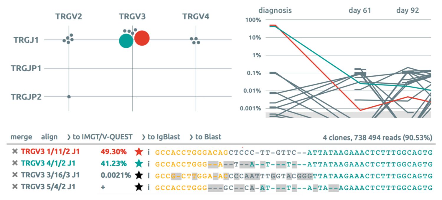
The first thing to be done is to see if some clonotypes should be clustered (because of sequencing or PCR errors for instance). This step could be automatized but, in any case, the automatic clustering would need to be checked by an expert eye.
By default in the bottom plot (the grid), the clonotypes are displayed according to their V and J genes (or more generally to their 5’ and 3’ genes).
44. Identify in the grid the clonotypes with an IGHV-3-13 IGHJ6 recombination and select them all. You can do so either by holding Ctrl or by drawing a rectangle around the clonotypes while maintaining down the left button of the mouse.
The sequences of the clonotypes now appear in the bottom part of the browser (the sequence panel). If many clonotypes are selected you can view more sequences by clicking on the flat up arrow in the middle of menu bar of sequence panel.
Then, the sequences in the sequence panel can be visually compared but you can also align them to see more easily their similarities.
45. Click on the Align button on the left-hand side. The differences are emphasized in bold.
Now it is the user’s expertise to determine if sequences are sufficiently similar, depending on her or his specific question. An efficiant hint to do so is to show the quality of each base of the Vidjil windows (menu sequence feature/quality). We can easily consider that sequence with a mismtach but with a poor quality at this position is a sequencing artifact and could be considered as identical of the support clonotype. If some sequences don’t appear to be similar enough, you can remove them from the sequence panel by clicking on the cross in front of the sequence in the sequence panel.
46. Remove all the sequences that are not similar enough with the first one.
Now all the sequences in the sequence panel should be highly similar. All their differences could be due to sequencing or PCR errors. These artifacts (mutations, homopolymers, insertions, deletions) depend on the sequencer and the PCR technique.
47. Cluster all those clonotypes in a single clonotype by clicking on the “Cluster” button, next to the Align button.
All the clustered sequences now appear within a same clonotype. That can be seen in the list: the clonotype which hosts the subclonotypes appears with a + on its left. You can click on the + to see the subclonotypes that have been clustered in the main one.
48. Click on the + and observe the changes in the grid.
As you may have noticed the subclonotypes appear again in the grid. You can compare their sequences again if you’d like (for example to double check that you were right to cluster them). You can also remove some subclonotypes from the cluster by clicking on the cross at their left in the list.
49. For the sake of the exercise, remove the last clonotype of the cluster.
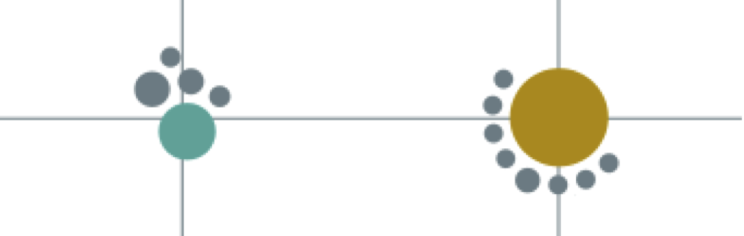
50. Open the cluster menu at the top of the page, and choose cluster by V/5. What happened ? There are now two clonotypes with TRGV2. Why ? These two clonotypes have been clustered on their V gene, but they differ by their allele. You can verify this by changing scatterplot preset by ‘V/J (allele)‘.
51. In the cluster menu, select revert to previous clusters to undo these clusterings.
You can show primer positions on the sequence according to predefined primer sets (Biomed-2 and EuroClonality-NGS by default), and display Genescan-like graph using the distance between these positions. When the primers are not found in the consensus sequence, their position is extrapolated from the germline sequence.
52. Select the preset Primers gap and observe the starting position of each clonotype.
53. Open the settings menu and select the primer set Biomed2.
This step is computationally intensive and apply on each clonotype of the analysis. More samples you have, more time it will take to finish.
54. You should now see a Genescan-like plot.
This plot show only top clontypes, limited to the top 100 by default.
55. Change the color by value with Locus. What do you see ?
56. Change the primer set to Euroclonality-NGS. What happens ?
Remark that some clonotypes become undefined. This happens for some particular segment, as IGH J6 .
As a proxy to sequence similarity we used the V and J genes, however there are other ways to assess sequence similarity that may be more pertinent. Moreover you may want to plot other metrics of the lymphocyte population. For instance we can choose to plot the V genes versus the length of the N insertions.
57. Go to the plot menu (in the upper left corner of the grid), and in the preset box choose V/N length.
Then you can continue aligning and clustering clonotypes if necessary.
58. You can also try the preset read length/GC content which tends to separate quite nicely the distinct clonotypes.
Note that you can choose any axis to be plotted: just go the plot menu and select any value you would like for the x axis and for the y axis. For bar charts, the box sizes always relates to the clonotype size, and the y axis selects the order of the boxes sharing a same x).
59. In the plot menu, switch between the “bubble plot” and the “bar plot”. In the bar plot mode, pass the mouse over the bars: What happens?
60. Press the keys 0 to 9 on the numeric keypad. What happens ? This switches the grid preset. Use shift + number to access to presets 10-19.
There is still a feature to help you analyse your data that we have not explored yet. You can change the colors to make it represent some variables of interest with the color by menu.
61. First choose the preset V/J (genes) and then color by N length (in the box at the top of the screen).
We apologize to color blinds: the colors are not yet color-blind friendly.
62. Choose now the preset CDR3 length distribution and then color by size. See that the color tiles in the info part (upper right) change to show the color key. Discrete axes (as tags) are shown with a selector. Some axes with many values (such as V and J genes) will not be displayed here. Continuous axes are shown with a radient color.
63. Instead of coloring by clonotype size, you could also color by clonotype. When coloring by clonotype, each clonotype has a random color. Thus in a bar plot, it is a convenient color mode to see the peaks that are due to a single clonotype or to several clonotypes. However clonotypes may be very similar. Another option is to color by CDR3. In such case all clonotypes with the same CDR3 will have the same color (note that, due to a lack of available colors two different CDR3s could share the same color just by chance).
Using those different features you should be able to analyse how similar your sequences are, and potentially you could cluster them if you’d like or tag them.
64. Select the most abundant clonotype. It now appears in the sequence panel. Now we would like to compare the sequence with the germline genes. We can add the germline genes to the sequence panel by going to the import/export menu and by clicking on add germline genes. Now we can click on the align button to see the alignment between the genes and the sequence. Mutations can be identified and silent mutations are displayed with a double border in blue.
This part is specific to samples analyzed with Vidjil-algo.
Some clonotypes may be less trustable than other ones… Let’s see how to spot them.
65. In the clonotype list, search clonotypes with an orange warning at the right side. Click on the warning. What are the warnings due to?
There may have several reasons:
average coverage: in that case the clonal sequence displayed is short compared to the reads in the clonotype. This may be the case when too different sequences have been put in a clonotype. The value is generally ≥ 80%.
e-value: It is a statistical value computed to ensure that recombinations have not been spot by chance. This value is generally much lower than 1 (< 10-5).
Clonotype similar to another one: In that case Vidjil-algo tells you that other clonotypes have the same genes and may be similar
Several genes with equal probability: The algorithm found several alleles or genes with the exact same e-value. This may happen when the sequence is too short.
Non-recombined sequences: Some known unrecombined sequences are tagged so that you can spot them easily. We tag the unrecombined IGHD7-27/IGHJ1 sequences that may be amplified.
You can view those values for any clonotype by clicking the i icon on the right side, in the list of clonotypes.
The existing warnings are listed on www.vidjil.org/doc/warnings/.
When you select a clonotype, you first see, in the aligner, the DNA sequence and its V, (D), and J segments. Next to the "align" button, several menus allow to display more features or information about the sequences. We will explore those menus.
66. Select the first clonotypes both in IGH and TRG. Then in the Data columns menu (the first on the left after the align button), click on productivity.
67. Now, click on the spin icon.
This queries external tools to process the selected sequences (as for example IMGT/V-QUEST) and, after a short time, will add the results to the clonotypes (as for example productivity computed by IMGT/V-QUEST, which is displayed by default).
Contact us if you need to query other software.
68. Open the sequence feature menu (the one before the last button). Click on "CDR3" and "quality".
In the aligner, there are now two new overlays on sequences. Above the sequence, the CDR3 is shown (you may have to move the horizontal scrollbar to view the CDR3). Under the sequence, the base quality of each position is shown, with a gradient color, from green (high quality) to red (low quality). The quality is shown for the window centered on the CDR3.
When aligning sequences, the quality color may help you to discriminate between potential biological mutations and sequencing errors (note that the current dataset is quite old and was sequenced with Ion Torrent, now the quality is usually much better).
Note that some features, such as primers or IMGT productivity, are available only after some additional computations.
First make sure to come back to the preset V/J (genes) in the plot menu.
If you want to focus on specific locus, you can click on the locus name in the upper left part. One click will make the locus disappear, another one will make it appear again. If you hold the Shift key (the one which is usually above the left Ctrl key) while clicking it will hide all the loci but the one you clicked on.
69. Click on IGH, while holding the Shift key. Now what is the number of analyzed reads? Why did it change?
70. Now click on TRG, to filter it in again.
71. Press on the g key. What happens? Now, press on the h key. Press on the g again (you can do that anytime you like :)). Let’s stick to the TRG locus.
You can also change the current locus by clicking on the locus name in the right part of the grid.
Sometimes you may include spike-ins in your sample to allow a more reliable quantification. Let us assume that the main clonotype with IGHV-3-9 / IGHJ5 is a spike-in whose expected concentration is 1% (.01).
72. First let’s color this clonotype with the standard tag.
73. Now we will set its concentration to 1% as expected. Click again on the star. In the normalize to field enter 1 and click ok. Now, in the graph, this clonotype should correspond to a straight line at 1%.
74. Notice how the concentrations of the other clonotypes have changed accordingly. You can go to the settings menu to disable this normalization and to go back to the raw concentrations.
Then you can set expected concentrations for other clonotypes and you are free to switch between those normalizations. It is also possible to set up normalization against external data, contact us if you are interested.
Please note that we have more advanced features to include your own spike-ins and to take into account spike-ins for different gene families. Contact us if you are interested.
Load now some data with several samples, such as again the Demo LIL-L3 dataset. The time graph shows the evolution of the top clonotypes of each sample into all the samples. Bear in mind that to ensure readability at most 10 curves are displayed in this graph by time point. When loading data with only one sample, the time graph is replaced by a second bar/grid plot.
75. Pass the mouse over the bubbles in the grid or over the lines in the time graph. Click on some clonotype. What happens ?
76. Click on the label of the time graph to select another sample. What happens to the number of analyzed reads ? to the size of the top clonotypes ?
When switching the time point, the views dynamically update which allows to easily track the changes along time. Also note that the number of analyzed reads differ from the previous point. We can again analyse the reason why some reads were unsegmented.
77. Hover labels of the time graph. What are you seeing ?
We will look now at how the V gene distribution evolves along the time.
78. In the grid, select the preset V distribution. Then click on the play icon in the upper left part (below the i icon).
By doing so you can look at how the V distribution changes along the time. Of course you can also change the data displayed in the grid to look at the evolution of another information.
We remind that by default at most 50 clonotypes are displayed on the time graph. However the remaining of the application usually displays the 50 most abundant clonotypes at each sample (which can account to hundreds of clonotypes, when having several samples).
79. Select a sample, order the list by size, and pass the mouse through the list of top 50 clonotypes. What happens in the graph when hovering clonotypes that are not in the top 50 ?
If you have many samples, you may wish to reorder the samples.
80. Drag the label of one sample to reorder the samples.
It is possible to hide some samples to have a better view of your analysis. This can be very useful to hide for example samples without a clonotype. Another case of usage is to load a run analysis with a lot of samples, and to restrict the list of active samples to retain only one that share a particular clonotype.
Open the menu to the upper right corner of graph. you can see that their are 3 buttons and 5 entries in the list corresponding to the list of samples. See the effet of the button here The name dispayed in the list is set accordingly with the settings choice for samples key.
81. Hover a sample name in the list. See what happens.
82. In this box, click on the entry labeled LIL-L3-3. When you have many samples this is another way to switch samples as sample names in the graph may be hardly readable in such a case.
It is also possible to hide/show a sample by clicking on the checkbox, by double clicking on the line, or by double clicking on the label in the timeline graph.
You may also want to compare two samples, either to check a replicate, to check for possible contaminations, or to compare different research or medical situations.
83. In the color by menu, choose Size. Select a different sample. What happens ? Are there some clonotypes with a significant different concentration in both samples ? Revert the color by choosing by tag.
Another option is to directly plot a log-log curve comparing two samples.
84. In the plot menu, choose the preset compare two samples. Click successively on two labels in the time graph to select the samples to be compared. Are there again some clonotypes with significant different concentrations in both samples ?
For some studies, VDJ designations are very important. In the list and in the sequence panel, those designations are written in their short form.
85. Put the mouse cursor over a clonotype. In the status bar (between the grid and the sequence panel), the complete designation appears.
We can double check this designation with other popular software.
86. Select a few clonotypes of the same locus. This requires an internet connection.
87. Click on the spin icon in the aligner panel header (the rightmost icon of the left part). The clonotype sequences are sent to IMGT/V-QUEST and the results from IMGT/V-QUEST are automatically retrieved by Vidjil. Once the spin icon changes to a tick, the informations have been successfully obtained.
88. Then, go to the next menu on the left and tick the checkbox [IMGT] V/D/J genes. In the sequence panel the boundaries of the V(D)J genes as computed by IMGT/V-QUEST are underlined. Thus you can compare the boundaries of the genes according to IMGT (underlined) and according to Vidjil (highlighted).
Note that data returned by IMGT/V-QUEST is available by clicking on the i icon of analyzed clonotypes, enabling you to compare the annotations made by the original software and by IMGT/V-QUEST.
89. Search a clonotype with sequence GCAGCCTAAAGGCTGAGGACACCCGACAGGGTATGGACGTCTGGGGCCAA and select it. Send this clonotype to IMGT/V-QUEST so that Vidjil retrieves the results in order to get the identity percentage of the V gene. Note this value for later comparaison.
90. As seen previously (see question 53), change the primer set to Biomed2 that is the set use for this sequencing.
91. Reopen the settings menu and check the line trim primers before external analysis. Relaunch IMGT and observe variation of the V identity percentage. What happened ?
92. You can also directly send the sequences to IMGT/V-QUEST, IgBlast, Blast or AssignSubsets by clicking the corresponding buttons in the External analysis menu. This opens a new page with the corresponding website.
It may happen the software makes a mistake in the VDJ designation. In such a case you’re very welcome to report us the problem and we will try to improve the designation algorithm.
93. Go in the Help menu and click on get support. It opens your mailer with a pre-composed email describing the data you are on as well as the clonotypes you selected..
Even if you do not use the get support button, it’s a good practice to send the complete address showing in your web browser, such as http://app.vidjil.org/?set=3241&config=39&plot=v,size,bar, when you want to discuss with colleagues or with us your data or your analyses.
Suppose that you would like to change the VDJ designation shown on the web application.
94. Click on the i icon in the list of clonotypes for the clonotype you want to change the designation. In the segmentation part, click the edit button. Choose what you would like to modify.
Beware: the modifications you made (name changes, clusters, clonotype tagging, sample reordering…) will not be automatically saved. You have to save your changes by yourself either by clicking on save patient in the top left menu (where the “patient” name is written) or by using the Ctrl+S keyboard shortcut. For this demonstration data, you cannot save your changes as you do not have the rights to modify this patient.
You can generate reports following predefined or custom templates, using different report sections to reflect the sample/disease you are analyzing.
95. In the export menu, open the report menu with export report.
We start with the default Full report. You can custom this report buy showing or hiding any sample, showing or hiding any locus, selecting the colors for all clonotypes and for selected clonotypes, updating the clonotypes you previously selected (with "star"), possibly removing them for the report, and finally adding, moving, or deleting *reports sections*, including plots you previously selected (within the “plot“ menu).
96. Close the report. Select clonotype by using the "star" button (status bar, bottom right), and "add to next report". Reopen the report menu. What happens?
97. Click on Show report button.
The generated report can be updated, commented, saved, or printed.
98. Hover inside a section. What are the four icons that appear in ?
Note that the modifications you have done there will apply to report sections on the main vidjil page.
Close the export menu and select the first time point and preset reads length distributions. Open the graphic menu and change axis X limits. Set it from 250 to 350. Click in this menu in button Add to next report. Regenerate a report and see the presence of this new section, with same limits. Note that this graphic keep on the selected time point at the moment of his creation.
Once you composed the report as you attended it to be for your purpose, you can choose to save it to found this preset next time, present in the preset list.
From export menu, multiple possiblities is offer to export analysis content.
top and bottom graphics: download a static image corresponding to the graphics view
csv: download detailed information on each clonotype, including ratio in complete or incomplete locus
fasta: open a new browser tab with selected clonotypes in fasta format plus their germline sequences. You can choose to copy/paste this content.
airr: download a CSV file that contains the clonotype detailed informations in AIRR format (see https://www.vidjil.org/doc/vidjil-algo/#airr-tsv-output). This format is shared by multiple repertoire analysis software.
Select the major TRG clonotypes of the last timepoint.
Note that the AIRR export file will contain only lines for the samples where the clonotype is present.
99. Select some clonotypes and align them. The alignment can be exported with the export aligned fasta button in the import/export menu.
Open a detailed description of it by clicking in the i icon present in the clonotypeq list row or in the segmenter panel if already selected (You can also open it by double clicking on it from the plot view).
At the line clonotype size, click on download icon and wait a little. A search is done inside the selected sample for the clonotype window and a file will be downloadable. This can take time.
Aurélien Béliard, Aurélie Caillault, Clément Chesnin, Marc Duez, Mathieu
Giraud, Tatiana Rocher, Mikaël Salson, Florian Thonier
support@vidjil.org